Important techniques for Deep Learning Models
Introduction
This blogpost is meant for those who are interested in the mathematical fundamentals behind the cutting-edge implementation practices in Deep Learning. The following sections are going to be purely theoretical with little to no coding application involved directly in contrast to my previous project-based posts. The main idea is to remove the mentality of “hiding behind libraries and abstractions” as opposed to using these to aid an overall research interest, with a certain level of necessary transparency in the understanding of the inner workings of standard models.
I will be covering the mathematical approach and aiming to develop an intuitive notion among the readers regarding three different practices - Learning Rate Calculation, Dropout and Batch Normalization. I consider these to be very relevant in the recent models which gives them the edge over standard training procedures.
Learning Rates
In the Deep Learning community, there has been a considerable amount of debate over what is the best way to go about calculating the learning rate for a model. In the following sections we shall look into three types of learning rate manipulations that provide better convergence and are adopted as the industry approach to neural networks.
First let’s talk about “Learning Rate Decay”. Learning Rate Decay is the formal term for the gradual reduction in learning rates as the epoch (training episode over the entire dataset) number rises. There are other implementations of learning rate decay (batch based), but epoch based LR decay is the most prominent. To understand why we would want our learning rate to decay is simple. Consider a situation where the learning rate is set to a value higher than it should be :
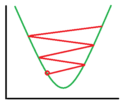
Or, in a higher dimensionality, it would look like something along these lines :
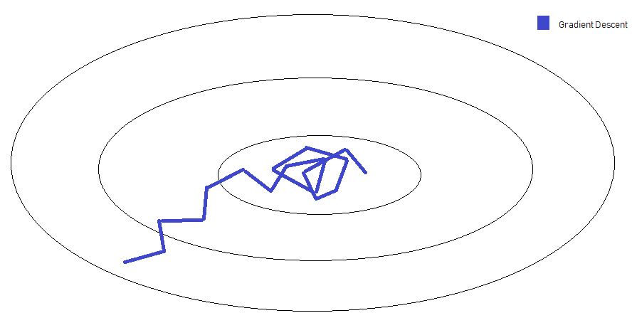
Clearly, we need to reduce our stepping size as we proceed closer to the minima point we desire to converge to. If our learning rate is unnecessarily slow from the beginning, our learning progress will be very slow and inefficient. Hence, we decay learning rates as we increase the amount of training our network has been exposed to. All these effects are summarised in the following illustration:
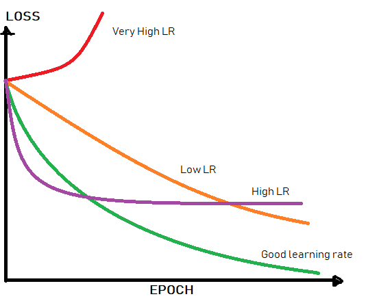
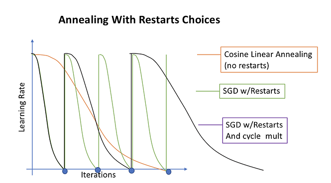
With LR Decay, we are combining the computational advantages of high learning rates initially, and the precisional supremity of low rates for convergence eventually. There are multiple decay (or annealing) implementations. They vary from linear, cosine, step-wise and exponential annealing based on epoch number.
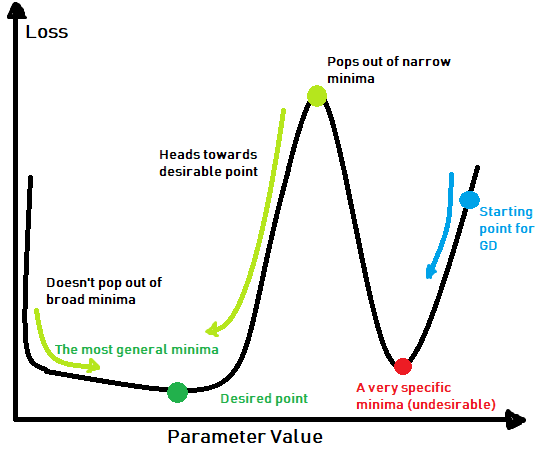
Let’s move on to more complicated annealing manipulations. Consider the following loss function:
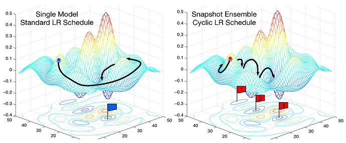
There are multiple points of minima (local) in this given surface. We want to reach a minima with a broader scope of low loss, meaning that sudden dips in an otherwise high loss are minimas that we want to avoid. For this, we reduce the learning rate over a given number of epochs (cycle_len), and then pop the LR back up to where it started, repeating this over and over again. Sometimes, we increase the number of epochs from cycle to cycle by some factor, as training proceeds further (cycle_mult).
This is done to pop out of the narrow dips in a given loss function, as the optimiser would reach a high value in such dips after the learning rate is increased back up, and not head down the same minima again. If the optimiser reaches close to a desired broad low loss minima, popping the learning rate back up has no impact, as the optimiser would again start heading back to the same minima (similar to osciallting around a minima with large learning rate), which is where we want to converge to. Eventually, as the learning rate decays for the final time, we would arrive at the desired convergence point. This is an effective way of dealing with non-convex optimisation problems.
The maximum learning rate calculation is fairly simple. We take a random starting point (weights initialisation) and apply learning rates starting from 0, recording the loss. Wherever we find the rate of decrease in loss to be the highest, we approximate that to be the learning rate cap for annealing with cycles. The same procedure is applicable to simple LR decay’s starting rates as well.
There are other learning rate optimisations includeing layer-wise optimisations, and adaptive rates for each conncetion in a network, but these are too nuanced, and follow the same fundamental principles that I have explained in this post. That’s about it for learning rates!
Dropout
Overfitting is a primary concern in medium to large neural networks. No dataset is a perfect representation of all possibilities that could be encountered by a neural network when making predictions. Overfitting leads to EXACT representation of the parameter-loss relationship between the network and the GIVEN data. This implies that when the network encounters data that is slightly deviated from the training dataset, it’s accuracy suffers a considerable drop.
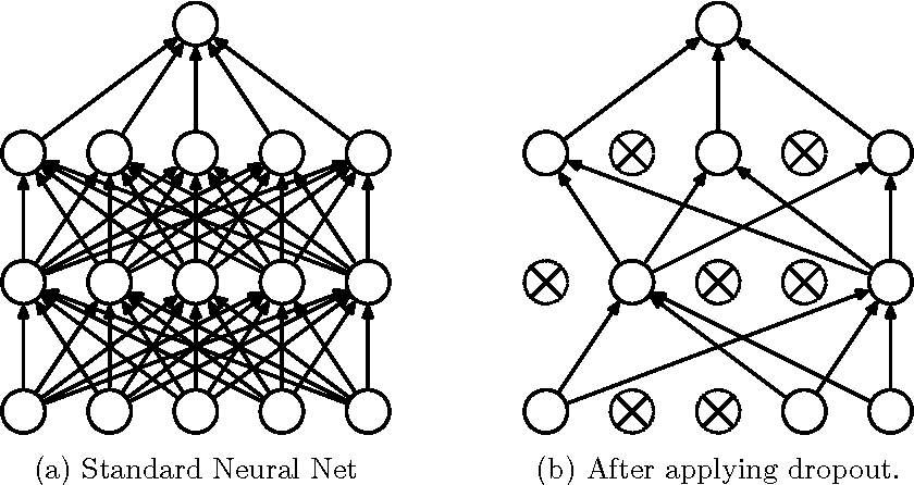
Dropout, much like L1 and L2 regularization, is a technique that is implemented to prevent overfitting in neural networks. In simple terms, dropout refers to “cutting-off” some nodes from the network at random (or pseudo-randomly), during a given forward and backward pass. More technically, At each training stage, individual nodes are either dropped out of the net with probability p or kept with probability 1-p, so that a reduced network is left; incoming and outgoing edges to a dropped-out node are also removed.
A given dataset might have biases with respect to one given feature, which might not apply to all kinds of data of the given situation. There might be co-dependencies among features and hidden nodes which we DO NOT want the network to learn, as these are specific to the training data, and not applicable to the general scenario. Dropout does the exact job of preventing such unwanted co-dependencies to be learned, and forces the network to understand the dataset in a more robust and generalized sense. In every forward and backward pass, the nodes cannot assume the presence or absence of any other node, achieving a relatively more independant form of learning. It creates a randomly “crippled” version of the neural network and forces learning upon it.
Another key feature of dropout is that the probability of shutting a node off from the main network can be individually chosen. By this, I mean to say that whichever layer is the largest in terms of connections and node size, can be forced with a dropout of higher probabilities than layers where overfitting is not that much of a concern. This is because most of the fitting and overfitting happens in the largest layers of the network. The output layer is always given a dropout of zero, as we want the prediction to be spanning the entire intended dimensions.
The math behind dropout is pretty straightforward. During training, in every given forward and backward pass, every hidden layer is given a “binary mask” containing 1’s and 0’s for respective nodes chosen to be active and shut off respectively (the mask will be random with probability ‘p’ for 0 to be multiplied with a given node). In forward pass, the hidden layer is then scalar-mutiplied by this mask, along with standard activation functions with the previous layer as input. This leads to the mask being applied in backprop as well, due to the chain rule of differentiation. This ensures that the same nodes are inactive during a given forward pass and backpropagation as well. The mask is then regenerated for the next pass, and the process is repeated.
During testing time, we simply replace the binary mask vector with the expectation vector. This means that if ‘p’ was 0.5, the mask will now be replaced with a vector containing 0.5 for every node in that given layer of nodes. This can be shown rigourously to be equivalent to a geometric mean for all the reduced neural networks generated with the binary masks, and can be thought of as the “average neural network” for the given dropout regularization.
A disadvantage of dropout is that the loss function is not stable in definition, as the parameters internally are vaninishing and coming into existence. This leads to a slower convergence which is slightly unstable in nature but each forward and backward pass is faster, as some nodes are not functional. The results after convergence are more generalized, as was the whole point. Keras has a really simple way of implementing dropouts in their models (just 1 additional line of code to the model per layer), and I urge the reader to try training a simple CNN on MNIST with and without dropout to see the difference.
Batch Normalisation
To understand why Batch Normalisation was proposed, let’s first understand the simple procedure of noramlising a given set of values.
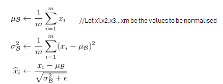
This generates a set of “nomarlised” datapoints with a mean of 0 and standard deviation 1. The feature-space that is fed into a neural network is usually normalised (not necessarily true always, because normalisation does lead to loss of information regarding units,magnitudes etc.). The reason behind doing so is that normalisation helps in improving the stability of the optimization algorithms that the data and the weights are being exposed to. A large variation in values of a given feature, and similary between the simultaneous values of different features leads to large variations in the weights and activations between the layers of the network, which can eventually lead to learning instability because of exploding gradients and a considerably volatile loss-function in general.
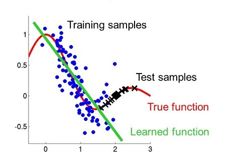
Another problem faced by neural networks (even with feature data normalisation) is the problem of “Covariate Shift”. This problem occurs when the network is shown and trained on a given dataset, and a more generalised form of the data is being tested on. The neural network shows less accuracy if the testing dataset is not a close representation of the training data, even if the two datasets will be classified with a constant function-apporximation. It is known as covariate “shift” because the generalised data might be a sort of shifted extension to the training dataset. The neural network cannot be expected to approximate the correct function with the not-so-general training dataset. Input data normalisation helps tackle this issue by making sure that the inputted information is not too vastly varied, maning that the feature-map of the data is closely clustered, and hence, easier to approximate with networks.
This is an inherent internal problem of neural networks as well. During training, assuming a neural network of 4 layers, the data that the third layer is being trained on, keeps changing as the parameters of the layers preceeding that are subjected to change with the optimization algorithm in play. It’s clear that there is an internal covariate shift of training data in between the layers of the network. Just like how input data normalisation helps in reducing external covariate shift, Batch Normalisation helps in reducing this internal problem. The data coming from the previous layer, before being subjected to the activation function of the layer in concern, is normalised, scaled up and shifted by learnable paramaters. This makes sure that the data has a fixed mean and variance as long as the shifting and scaling parameters are not being changed. When they are, this change is gradual, and hence the network doesn’t see a sudden change in data clusters, making learning a smooth and stable process.
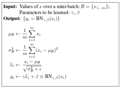
The above, is done layer-wise. The two parameters of scaling and shifting are layer-specific and learnable. The data is then activated with the layer’s activation function, and then fed into the next layer. The “batch” aspect comes into the picture because the above alogithm is implemented on mini-batches of the overall training data. During testing time, a weighted exponential average of the means and standard deviations is used for each layer, across all the mini-batches encountered during training along with the the learned beta and gamma paramters (for each layer, again.). This how testing data is generally noramlised. Another way is to calculate the mean and deviation for each layer for the entire data available, but this is computationally expensive for deep networks, making the latter more viable.
BatchNorm increases training speeds, allows for higher learning rates to work stably, and also provides some regularisation effect because normalisationa dds some noise to data (although this is not the primary intention). Most deep learning frameworks come with in-built BN enabling features, making it a solid implementation procedure for practitioners.
Suggested Readings and Sources
- http://forums.fast.ai/t/deeplearning-lecnotes2/7515
- https://arxiv.org/pdf/1506.01186.pdf
- https://www.youtube.com/watch?v=QzulmoOg2JE
- https://arxiv.org/pdf/1206.1106.pdf
- https://www.kdnuggets.com/2017/11/estimating-optimal-learning-rate-deep-neural-network.html
- https://www.youtube.com/watch?v=dXB-KQYkzNU
- https://arxiv.org/abs/1502.03167
- https://medium.com/deeper-learning/glossary-of-deep-learning-batch-normalisation-8266dcd2fa82
- https://www.youtube.com/watch?v=nUUqwaxLnWs
- https://medium.com/@amarbudhiraja/https-medium-com-amarbudhiraja-learning-less-to-learn-better-dropout-in-deep-machine-learning-74334da4bfc5
- https://machinelearningmastery.com/dropout-regularization-deep-learning-models-keras/
- https://www.youtube.com/watch?v=ARq74QuavAo
- https://www.youtube.com/watch?v=UcKPdAM8cnI </ul